We are working with XX-Large resources on ARE (28 cores, 126 GB)
[2]:
#Set up a dask distributed client, so that chunks of data can be sent and# processed by different cores/"workers".# Click "Launch dashboard in JupyterLab" within this cell's output to see dask progressclient=Client(threads_per_worker=1)client
AUS2200 catalog with 1 dataset(s) from 244 asset(s):
unique
path
244
file_type
1
realm
1
model_id
1
experiment_id
1
frequency
1
variable_id
1
version
1
time_range
244
derived_variable_id
0
[4]:
#Define lat lon slices, equivalent to almost the entire AUS2200 domainlon_slice=slice(108,159)lat_slice=slice(-45.7,-6.831799)# Single model level (111.7 m)lev_slice=slice(100,120)#Define times to slicestart_time="2016-01-01 00:00"end_time="2016-02-01 00:00"
Previous versions of this notebook we specified the chunks as {"time":6,"lat":-1,"lon":-1,"lev":{}}. For lat and lon, "-1" means that the chunk sizes in those dimensions (1963 for lat, 2574 for lon) are equivalent to the length of the dimensions. In other words, the dataset is not chunked up in those dimensions.
However, the dataset is chunked along time (with a chunk size of 6). This is the best we can do for AUS2200 as each file is 6 time steps long. We can rechunk the time dimension later by calling aus2200_ta.chunk({"time":chunksize}), but this can be very slow.
Our aim is to have small enough chunks to fit on memory, but large enough chunks to reduce the time taken to pass data between workers and to reduce the number of operations dask is doing. The chunk size here (115 MB) is okay, with around 200 MB being a pretty good aim (although there is no standard rules around what chunk sizes are optimal, it takes some experimenting)
Advances in the xarray/dask ecosystem means that you can now typically just specify chunks="auto" to have dask figure out (close to) optimal chunks for you. Intake takes care of this for us.
Now we’d like to compute a rolling daily average temperature. Rolling operations can be very slow, because for each point we need to access neighbouring time chunks
[7]:
time_window=24#equivalent to one day for the hourly data heremin_periods=12#for each time step, there must be at least 12 hours in the moving window# for the rolling mean to be defined.aus2200_ta_daily_mean=aus2200_ta.rolling(dim={"time":24},center=True,min_periods=12).mean()
[8]:
aus2200_ta_daily_mean
[8]:
<xarray.DataArray 'ta' (time: 744, lev: 1, lat: 1963, lon: 2575)> Size: 15GB
dask.array<getitem, shape=(744, 1, 1963, 2575), dtype=float32, chunksize=(42, 1, 424, 520), chunktype=numpy.ndarray>
Coordinates:
  * time     (time) datetime64[ns] 6kB 2016-01-01T01:00:00 ... 2016-02-01
  * lev      (lev) float64 8B 111.7
  * lat      (lat) float64 16kB -45.7 -45.68 -45.66 ... -6.891 -6.871 -6.852
  * lon      (lon) float64 21kB 108.0 108.0 108.1 108.1 ... 158.9 159.0 159.0
Attributes:
    standard_name:          air_temperature
    long_name:              Air Temperature
    comment:                Air Temperature
    units:                  K
    cell_methods:           area: mean time: point
    cell_measures:          area: areacella
    coverage_content_type:  modelResult
Note that dask hasn’t done anything yet because we haven’t actually needed to access any data (with only metadata shown above so far). When we start making plots in the following cells, then dask will actually start doing computations and loading the required data into memory.
If for some reason we would like all the data in memory to access it, we can use compute() or persist() commands, such as
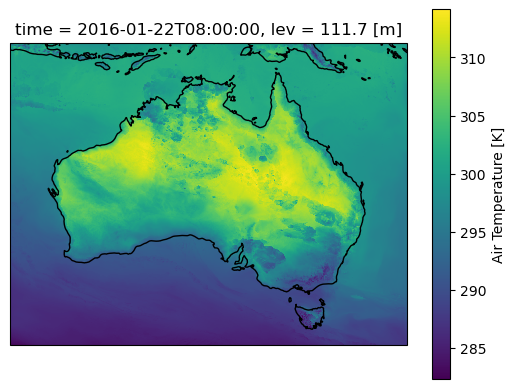
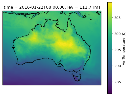
Lets plot a single time step and start some computations. Note that the daily mean here smooths out small variations compared with the original temperature field
[9]:
#First for the original air temperature dataax=plt.axes(projection=ccrs.PlateCarree())aus2200_ta.sel(time="2016-01-22 08:00").plot()ax.coastlines()
[9]:
<cartopy.mpl.feature_artist.FeatureArtist at 0x15115ccff830>
[10]:
#And for the rolling daily meanax=plt.axes(projection=ccrs.PlateCarree())aus2200_ta_daily_mean.sel(time="2016-01-22 08:00").plot()ax.coastlines()
/g/data/xp65/public/apps/med_conda/envs/analysis3-26.05/lib/python3.12/site-packages/distributed/client.py:3387: UserWarning: Sending large graph of size 10.43 MiB.
This may cause some slowdown.
Consider loading the data with Dask directly
 or using futures or delayed objects to embed the data into the graph without repetition.
See also https://docs.dask.org/en/stable/best-practices.html#load-data-with-dask for more information.
  warnings.warn(
[10]:
<cartopy.mpl.feature_artist.FeatureArtist at 0x1512247495e0>
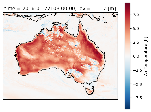
Now calculate the temperature perturbations relative to the daily mean. Perturbations will re-introduce and highlight small-scale factors like convective cold pools and sea breezes along the coast, as well as allowing us to quantify the diurnal cycle.
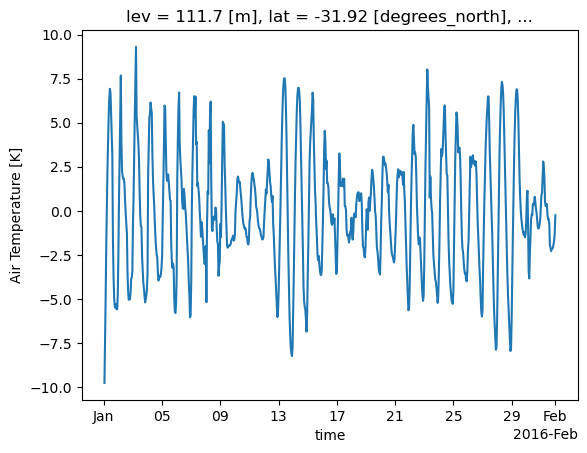
As above, but for temperatue perturbations. Also plot for a single lat/lon location for the entire month
Note that the time series computation takes a lot longer, because dask needs to access many more files on disk (AUS2200 data is saved in 6-hourly files as discussed earlier)
/g/data/xp65/public/apps/med_conda/envs/analysis3-26.05/lib/python3.12/site-packages/distributed/client.py:3387: UserWarning: Sending large graph of size 12.65 MiB.
This may cause some slowdown.
Consider loading the data with Dask directly
 or using futures or delayed objects to embed the data into the graph without repetition.
See also https://docs.dask.org/en/stable/best-practices.html#load-data-with-dask for more information.
  warnings.warn(
[12]:
<cartopy.mpl.feature_artist.FeatureArtist at 0x1512271114f0>
[13]:
# This does not work: see https://github.com/dask/dask/issues/12198try:aus2200_ta_daily_pert=aus2200_ta_daily_pert.sel(lat=-31.9275,lon=115.9764,method="nearest").plot()exceptValueError:print("Failed due to dask/bottleneck issue... see below for fix")
/g/data/xp65/public/apps/med_conda/envs/analysis3-26.05/lib/python3.12/site-packages/distributed/client.py:3387: UserWarning: Sending large graph of size 12.77 MiB.
This may cause some slowdown.
Consider loading the data with Dask directly
 or using futures or delayed objects to embed the data into the graph without repetition.
See also https://docs.dask.org/en/stable/best-practices.html#load-data-with-dask for more information.
  warnings.warn(
2026-05-15 12:21:50,962 - distributed.worker - ERROR - Compute Failed
Key:       ('getitem-overlap-_trim-9debcf9e98eb529079aaf1b071f41466', 0, 0, 2, 0)
State:     executing
Task:  <Task ('getitem-overlap-_trim-9debcf9e98eb529079aaf1b071f41466', 0, 0, 2, 0) _execute_subgraph(...)>
Exception: "ValueError('Moving window (=24) must between 1 and 23, inclusive')"
Traceback: ''
Failed due to dask/bottleneck issue... see below for fix
Because of an annoying bug in dask >= 2024.11.0, we have to do a bit of a workaround here.
We’re going to select our point, and then instantiate the whole array in memory, so that we don’t touch dask, instead delegating the work to numpy.
This is generally inadvisable - it’s okay for a single point though, because we probably don’t have that much data
If you try to do this with a large 3/4D array, you will probably run out of memory.
# This array is only 3KB - so we can load it all into memoryperth_ta=perth_ta.compute()
[16]:
# And now we can redo the rolling mean without any issuesperth_ta_daily_mean=perth_ta.rolling(dim={"time":24},center=True,min_periods=12).mean()perth_ta_daily_pert=perth_ta-perth_ta_daily_mean
[17]:
perth_ta_daily_pert.plot()
[17]:
[<matplotlib.lines.Line2D at 0x1511373b2ff0>]
Andrew Brown
ARC Centre of Excellence for 21st Century Weather, University of Melbourne
Samuel Green
ARC Centre of Excellence for 21st Century Weather & Climate Change Research Centre, UNSW Sydney
Charles Turner
ACCESS-NRI, Australian National University, Canberra
If you have any enquries, suggested improvements or bug reports related to this recipe, please open an issue or start a discussion in this repository.