Demo for the AUS2200 intake catalogue

How to load output for an experiment without knowledge where the output lives on NCI

import intake
import cf_xarray

catalog = intake.cat.access_nri['AUS2200']

# Until https://github.com/ACCESS-NRI/access-nri-intake-catalog/pull/621 is merged
catalog = catalog.unwrap()

You can also explore datasets in the intake catalog via https://access-nri.github.io/interactive-data-catalogue/#/, which will give you an interactive way to explore them in a browser

List all the datasets available.

list(catalog)[:5]

['f.AUS2200.6hrPlev.zg.v1-0',
 'f.AUS2200.1hr.pfull.v1-0',
 'f.AUS2200.1hr.rsdsdiff.v1-0',
 'f.AUS2200.1hr.hus.v1-0',
 'f.AUS2200.1hr.va.v1-0']

# This is not very helpful - so lets figure out what is in the datastore

catalog

AUS2200 catalog with 61 dataset(s) from 21471 asset(s):

	unique
path	21471
file_type	1
realm	2
model_id	1
experiment_id	16
frequency	6
variable_id	48
version	1
time_range	2054
derived_variable_id	0

# experiment_id looks like it might be helpful!
catalog.unique().experiment_id

['mjo-lanina2018',
 'mjo-elnino2016',
 'coralsea-sstreduced',
 'ashwed1983',
 'mjo-neutral2013',
 'canberra2003',
 'flood2022',
 'ashwed1980',
 'ecoastlow-corclimsst',
 'blacksat2009',
 'ecoastlow-smooth',
 'ecoastlow-evolvsst',
 'ecoastlow-climsst',
 'ecoastlow-tasclimsst',
 'coralsea-sstobs',
 'ecoastlow-fixsst']

# Lets pick the Canberra 2003 experiment
experiment = catalog.search(experiment_id='canberra2003')

At the moment we have one dataset for each separate simulation and a combined dataset which includes all simulations.

Example of dataset for a single simulation: canberra03

# Lets pick the Canberra 2003 experiment
experiment = catalog.search(experiment_id='canberra2003')
experiment

AUS2200 catalog with 56 dataset(s) from 341 asset(s):

	unique
path	341
file_type	1
realm	2
model_id	1
experiment_id	1
frequency	4
variable_id	47
version	1
time_range	35
derived_variable_id	0

What are the available variables?

experiment.unique()['variable_id']

['rainmxrat',
 'vas',
 'refl',
 'cl',
 'wa',
 'clmed',
 'clw',
 'ta',
 'cli',
 'grplmxrat',
 'hus',
 'pralsns',
 'eow',
 'theta',
 'tke',
 'uas',
 'hfss',
 'va',
 'pralsprof',
 'hfls',
 'ua',
 'pfull',
 'huss',
 'clmxro',
 'rsds',
 'mrsol',
 'psl',
 'rsdt',
 'reflmax',
 'estot',
 'wsgmax10m',
 'evspsbl',
 'lmask',
 'z0',
 'clhigh',
 'cllow',
 'rsut',
 'rss',
 'rsdsdir',
 'orog',
 'mrso',
 'tas',
 'zmla',
 'rlds',
 'rls',
 'rsdsdiff',
 'rlut']

Let’s get one (e.g., the temperature) and do some super-duper analysis!

ds = experiment.search(variable_id='tas', frequency="1hr").to_dask()
ds

<xarray.Dataset> Size: 2GB
Dimensions:    (time: 96, bnds: 2, lat: 2120, lon: 2600)
Coordinates:
  * time       (time) datetime64[ns] 768B 2003-01-16T00:29:59.999999872 ... 2...
  * lat        (lat) float64 17kB -48.79 -48.77 -48.75 ... -6.871 -6.852 -6.832
  * lon        (lon) float64 21kB 107.5 107.5 107.6 107.6 ... 158.9 159.0 159.0
    height     float64 8B ...
Dimensions without coordinates: bnds
Data variables:
    time_bnds  (time, bnds) datetime64[ns] 2kB dask.array<chunksize=(96, 2), meta=np.ndarray>
    lat_bnds   (lat, bnds) float64 34kB dask.array<chunksize=(2120, 2), meta=np.ndarray>
    lon_bnds   (lon, bnds) float64 42kB dask.array<chunksize=(2600, 2), meta=np.ndarray>
    tas        (time, lat, lon) float32 2GB dask.array<chunksize=(6, 2120, 2600), meta=np.ndarray>
Attributes: (12/57)
    Conventions:                     CF-1.7 ACDD1.3
    creation_date:                   2023-10-19T06:04:51Z
    data_specs_version:              01.00.00
    date_created:                    2023-06-05
    exp_description:                 A limited area model study of the entire...
    external_variables:              areacella
    ...                              ...
    intake_esm_attrs:frequency:      1hr
    intake_esm_attrs:variable_id:    tas
    intake_esm_attrs:version:        v1-0
    intake_esm_attrs:time_range:     200301160030-200301192330
    intake_esm_attrs:_data_format_:  netcdf
    intake_esm_dataset_key:          f.AUS2200.1hr.tas.v1-0

xarray.Dataset

• Dimensions:
  • time: 96
  • bnds: 2
  • lat: 2120
  • lon: 2600
• Coordinates: (4)
  • time
    (time)
    datetime64[ns]
    2003-01-16T00:29:59.999999872 .....

    bounds :

    time_bnds

    axis :

    T

    long_name :

    time

    standard_name :

    time

    array(['2003-01-16T00:29:59.999999872', '2003-01-16T01:30:00.000000000',
           '2003-01-16T02:30:00.000000128', '2003-01-16T03:29:59.999999872',
           '2003-01-16T04:30:00.000000000', '2003-01-16T05:30:00.000000128',
           '2003-01-16T06:29:59.999999872', '2003-01-16T07:30:00.000000000',
           '2003-01-16T08:30:00.000000128', '2003-01-16T09:29:59.999999872',
           '2003-01-16T10:30:00.000000000', '2003-01-16T11:30:00.000000128',
           '2003-01-16T12:29:59.999999872', '2003-01-16T13:30:00.000000000',
           '2003-01-16T14:30:00.000000128', '2003-01-16T15:29:59.999999872',
           '2003-01-16T16:30:00.000000000', '2003-01-16T17:30:00.000000128',
           '2003-01-16T18:29:59.999999872', '2003-01-16T19:30:00.000000000',
           '2003-01-16T20:30:00.000000128', '2003-01-16T21:29:59.999999872',
           '2003-01-16T22:30:00.000000000', '2003-01-16T23:30:00.000000128',
           '2003-01-17T00:29:59.999999872', '2003-01-17T01:30:00.000000000',
           '2003-01-17T02:30:00.000000128', '2003-01-17T03:29:59.999999872',
           '2003-01-17T04:30:00.000000000', '2003-01-17T05:30:00.000000128',
           '2003-01-17T06:29:59.999999872', '2003-01-17T07:30:00.000000000',
           '2003-01-17T08:30:00.000000128', '2003-01-17T09:29:59.999999872',
           '2003-01-17T10:30:00.000000000', '2003-01-17T11:30:00.000000128',
           '2003-01-17T12:29:59.999999872', '2003-01-17T13:30:00.000000000',
           '2003-01-17T14:30:00.000000128', '2003-01-17T15:29:59.999999872',
           '2003-01-17T16:30:00.000000000', '2003-01-17T17:30:00.000000128',
           '2003-01-17T18:29:59.999999872', '2003-01-17T19:30:00.000000000',
           '2003-01-17T20:30:00.000000128', '2003-01-17T21:29:59.999999872',
           '2003-01-17T22:30:00.000000000', '2003-01-17T23:30:00.000000128',
           '2003-01-18T00:29:59.999999872', '2003-01-18T01:30:00.000000000',
           '2003-01-18T02:30:00.000000128', '2003-01-18T03:29:59.999999872',
           '2003-01-18T04:30:00.000000000', '2003-01-18T05:30:00.000000128',
           '2003-01-18T06:29:59.999999872', '2003-01-18T07:30:00.000000000',
           '2003-01-18T08:30:00.000000128', '2003-01-18T09:29:59.999999872',
           '2003-01-18T10:30:00.000000000', '2003-01-18T11:30:00.000000128',
           '2003-01-18T12:29:59.999999872', '2003-01-18T13:30:00.000000000',
           '2003-01-18T14:30:00.000000128', '2003-01-18T15:29:59.999999872',
           '2003-01-18T16:30:00.000000000', '2003-01-18T17:30:00.000000128',
           '2003-01-18T18:29:59.999999872', '2003-01-18T19:30:00.000000000',
           '2003-01-18T20:30:00.000000128', '2003-01-18T21:29:59.999999872',
           '2003-01-18T22:30:00.000000000', '2003-01-18T23:30:00.000000128',
           '2003-01-19T00:29:59.999999872', '2003-01-19T01:30:00.000000000',
           '2003-01-19T02:30:00.000000128', '2003-01-19T03:29:59.999999872',
           '2003-01-19T04:30:00.000000000', '2003-01-19T05:30:00.000000128',
           '2003-01-19T06:29:59.999999872', '2003-01-19T07:30:00.000000000',
           '2003-01-19T08:30:00.000000128', '2003-01-19T09:29:59.999999872',
           '2003-01-19T10:30:00.000000000', '2003-01-19T11:30:00.000000128',
           '2003-01-19T12:29:59.999999872', '2003-01-19T13:30:00.000000000',
           '2003-01-19T14:30:00.000000128', '2003-01-19T15:29:59.999999872',
           '2003-01-19T16:30:00.000000000', '2003-01-19T17:30:00.000000128',
           '2003-01-19T18:29:59.999999872', '2003-01-19T19:30:00.000000000',
           '2003-01-19T20:30:00.000000128', '2003-01-19T21:29:59.999999872',
           '2003-01-19T22:30:00.000000000', '2003-01-19T23:30:00.000000128'],
          dtype='datetime64[ns]')

  • lat
    (lat)
    float64
    -48.79 -48.77 ... -6.852 -6.832

    bounds :

    lat_bnds

    units :

    degrees_north

    axis :

    Y

    long_name :

    Latitude

    standard_name :

    latitude

    array([-48.787998, -48.7682  , -48.748398, ...,  -6.871399,  -6.851597,
            -6.831799], shape=(2120,))

  • lon
    (lon)
    float64
    107.5 107.5 107.6 ... 159.0 159.0

    bounds :

    lon_bnds

    units :

    degrees_east

    axis :

    X

    long_name :

    Longitude

    standard_name :

    longitude

    array([107.519997, 107.539795, 107.559593, ..., 158.940598, 158.960388,
           158.980194], shape=(2600,))

  • height
    ()
    float64
    ...

    units :

    m

    axis :

    Z

    positive :

    up

    long_name :

    height

    standard_name :

    height

    [1 values with dtype=float64]

• Data variables: (4)
  • time_bnds
    (time, bnds)
    datetime64[ns]
    dask.array<chunksize=(96, 2), meta=np.ndarray>

    Array Chunk Bytes 1.50 kiB 1.50 kiB Shape (96, 2) (96, 2) Dask graph 1 chunks in 2 graph layers Data type datetime64[ns] numpy.ndarray

  • lat_bnds
    (lat, bnds)
    float64
    dask.array<chunksize=(2120, 2), meta=np.ndarray>

    Array Chunk Bytes 33.12 kiB 33.12 kiB Shape (2120, 2) (2120, 2) Dask graph 1 chunks in 2 graph layers Data type float64 numpy.ndarray

  • lon_bnds
    (lon, bnds)
    float64
    dask.array<chunksize=(2600, 2), meta=np.ndarray>

    Array Chunk Bytes 40.62 kiB 40.62 kiB Shape (2600, 2) (2600, 2) Dask graph 1 chunks in 2 graph layers Data type float64 numpy.ndarray

  • tas
    (time, lat, lon)
    float32
    dask.array<chunksize=(6, 2120, 2600), meta=np.ndarray>

    standard_name :

    air_temperature

    long_name :

    Near-Surface Air Temperature

    comment :

    near-surface (for access 1.5 meters) air temperature

    units :

    K

    cell_methods :

    area: mean time: mean

    cell_measures :

    area: areacella

    history :

    2023-10-19T06:04:25Z altered by CMOR: Treated scalar dimension: 'height'. 2023-10-19T06:04:25Z altered by CMOR: replaced missing value flag (9.96921e+36) and corresponding data with standard missing value (1e+20).

    coverage_content_type :

    modelResult

    Array Chunk Bytes 1.97 GiB 126.16 MiB Shape (96, 2120, 2600) (6, 2120, 2600) Dask graph 16 chunks in 2 graph layers Data type float32 numpy.ndarray

• Attributes: (57)

  Conventions :

  CF-1.7 ACDD1.3

  creation_date :

  2023-10-19T06:04:51Z

  data_specs_version :

  01.00.00

  date_created :

  2023-06-05

  exp_description :

  A limited area model study of the entire Australian continent at 2.2 km resolution, using the UM atmospheric model. ERA5+ERA5Land reanalysis data was used to provide initial and boundary conditions. The study covers the time period of 2003-01-16 to 2003-01-19, including the 2003 Canberra bushfires.

  external_variables :

  areacella

  forcing :

  GHG, Oz, SA, Sl, Vl, BC, OC, (GHG = CO2, N2O, CH4, CFC11, CFC12, CFC113, HCFC22, HFC125, HFC134a)

  frequency :

  1hr

  geospatial_lat_max :

  -6.83

  geospatial_lat_min :

  -48.79

  geospatial_lon_max :

  158.98

  geospatial_lon_min :

  107.52

  grid :

  native atmosphere grid (2120x2600 latxlon)

  history :

  2023-10-19T06:04:51Z ; CMOR rewrote data to be consistent with , CF-1.7 ACDD1.3 and CF standards.

  institution :

  University of Melbourne

  keywords :

  Climate change processes, Adverse weather events, Cloud physics

  nominal_resolution :

  2.2 km

  organisation :

  Centre of Excellence for Climate Extremes

  product :

  model-output

  product_version :

  v1.0

  realm :

  atmos

  source :

  UM v12.2 ECMWF ERA5 and ERA5-Land reanalysis fields used as forcings

  source_id :

  AUS2200

  table_id :

  A1hr

  table_info :

  Creation Date:(20 June 2023) MD5:71a4110ed3210ee3a5e9f7f71551dad2

  time_coverage_start :

  2003-01-16

  tracking_id :

  ddbb400b-b0a9-41f9-b88c-ecbccfeff5d3

  variable_id :

  tas

  version :

  v1.0

  license :

  https://creativecommons.org/licenses/by/4.0/

  cmor_version :

  3.7.1

  title :

  AUS2200 Unified Model atmospheric simulation of the 2003 Canberra bushfire, over Australia at 2.2km resolution.

  experiment_id :

  canberra2003

  experiment :

  canberra2003

  creator_role :

  model simulation, post-processing, principal investigator

  creator_url :

  https://orcid.org/0000-0003-3952-6344, https://orcid.org/0000-0002-0164-5105, https://orcid.org/0000-0001-9499-5894

  contact :

  hooman.ayat@unimelb.edu.au

  comment :

  post-processed using ACCESS-MOPPeR v0.6.0 https://doi.org/10.5281/zenodo.10976467

  publisher_name :

  NCI

  publisher_email :

  help@nci.org.au

  creator_name :

  Dale Roberts, Paola Petrelli, Hooman Ayat

  creator_email :

  dale.roberts1@anu.edu.au, paola.petrelli@utas.edu.au, hooman.ayat@unimelb.edu.au

  time_coverage_end :

  2003-01-19

  id :

  https://doi.org/10.25194/vhs6-ja29

  citation :

  Roberts, Dale, Petrelli, Paola, Ayat, Hooman. AUS2200 Unified Model atmospheric simulation of the 2003 Canberra bushfire, over Australia at 2.2km resolution. v1.0 (2024). NCI Australia. (Dataset) https://doi.org/10.25914/vhs6-ja29

  intake_esm_vars :

  ['tas']

  intake_esm_attrs:path :

  /g/data/bs94/AUS2200/canberra2003/v1-0/1hr/tas/tas_AUS2200_canberra03_1hr_200301160030-200301192330.nc

  intake_esm_attrs:file_type :

  f

  intake_esm_attrs:realm :

  atmos

  intake_esm_attrs:model_id :

  AUS2200

  intake_esm_attrs:experiment_id :

  canberra2003

  intake_esm_attrs:frequency :

  1hr

  intake_esm_attrs:variable_id :

  tas

  intake_esm_attrs:version :

  v1-0

  intake_esm_attrs:time_range :

  200301160030-200301192330

  intake_esm_attrs:_data_format_ :

  netcdf

  intake_esm_dataset_key :

  f.AUS2200.1hr.tas.v1-0

tas = ds['tas']
tas

<xarray.DataArray 'tas' (time: 96, lat: 2120, lon: 2600)> Size: 2GB
dask.array<open_dataset-tas, shape=(96, 2120, 2600), dtype=float32, chunksize=(6, 2120, 2600), chunktype=numpy.ndarray>
Coordinates:
  * time     (time) datetime64[ns] 768B 2003-01-16T00:29:59.999999872 ... 200...
  * lat      (lat) float64 17kB -48.79 -48.77 -48.75 ... -6.871 -6.852 -6.832
  * lon      (lon) float64 21kB 107.5 107.5 107.6 107.6 ... 158.9 159.0 159.0
    height   float64 8B ...
Attributes:
    standard_name:          air_temperature
    long_name:              Near-Surface Air Temperature
    comment:                near-surface (for access 1.5 meters) air temperature
    units:                  K
    cell_methods:           area: mean time: mean
    cell_measures:          area: areacella
    history:                2023-10-19T06:04:25Z altered by CMOR: Treated sca...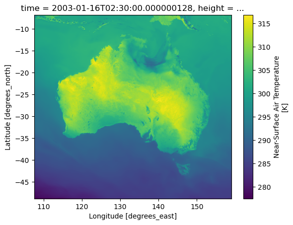
    coverage_content_type:  modelResult

xarray.DataArray

'tas'

• time: 96
• lat: 2120
• lon: 2600

• dask.array<chunksize=(6, 2120, 2600), meta=np.ndarray>

  Array Chunk Bytes 1.97 GiB 126.16 MiB Shape (96, 2120, 2600) (6, 2120, 2600) Dask graph 16 chunks in 2 graph layers Data type float32 numpy.ndarray

• Coordinates: (4)
  • time
    (time)
    datetime64[ns]
    2003-01-16T00:29:59.999999872 .....

    bounds :

    time_bnds

    axis :

    T

    long_name :

    time

    standard_name :

    time

    array(['2003-01-16T00:29:59.999999872', '2003-01-16T01:30:00.000000000',
           '2003-01-16T02:30:00.000000128', '2003-01-16T03:29:59.999999872',
           '2003-01-16T04:30:00.000000000', '2003-01-16T05:30:00.000000128',
           '2003-01-16T06:29:59.999999872', '2003-01-16T07:30:00.000000000',
           '2003-01-16T08:30:00.000000128', '2003-01-16T09:29:59.999999872',
           '2003-01-16T10:30:00.000000000', '2003-01-16T11:30:00.000000128',
           '2003-01-16T12:29:59.999999872', '2003-01-16T13:30:00.000000000',
           '2003-01-16T14:30:00.000000128', '2003-01-16T15:29:59.999999872',
           '2003-01-16T16:30:00.000000000', '2003-01-16T17:30:00.000000128',
           '2003-01-16T18:29:59.999999872', '2003-01-16T19:30:00.000000000',
           '2003-01-16T20:30:00.000000128', '2003-01-16T21:29:59.999999872',
           '2003-01-16T22:30:00.000000000', '2003-01-16T23:30:00.000000128',
           '2003-01-17T00:29:59.999999872', '2003-01-17T01:30:00.000000000',
           '2003-01-17T02:30:00.000000128', '2003-01-17T03:29:59.999999872',
           '2003-01-17T04:30:00.000000000', '2003-01-17T05:30:00.000000128',
           '2003-01-17T06:29:59.999999872', '2003-01-17T07:30:00.000000000',
           '2003-01-17T08:30:00.000000128', '2003-01-17T09:29:59.999999872',
           '2003-01-17T10:30:00.000000000', '2003-01-17T11:30:00.000000128',
           '2003-01-17T12:29:59.999999872', '2003-01-17T13:30:00.000000000',
           '2003-01-17T14:30:00.000000128', '2003-01-17T15:29:59.999999872',
           '2003-01-17T16:30:00.000000000', '2003-01-17T17:30:00.000000128',
           '2003-01-17T18:29:59.999999872', '2003-01-17T19:30:00.000000000',
           '2003-01-17T20:30:00.000000128', '2003-01-17T21:29:59.999999872',
           '2003-01-17T22:30:00.000000000', '2003-01-17T23:30:00.000000128',
           '2003-01-18T00:29:59.999999872', '2003-01-18T01:30:00.000000000',
           '2003-01-18T02:30:00.000000128', '2003-01-18T03:29:59.999999872',
           '2003-01-18T04:30:00.000000000', '2003-01-18T05:30:00.000000128',
           '2003-01-18T06:29:59.999999872', '2003-01-18T07:30:00.000000000',
           '2003-01-18T08:30:00.000000128', '2003-01-18T09:29:59.999999872',
           '2003-01-18T10:30:00.000000000', '2003-01-18T11:30:00.000000128',
           '2003-01-18T12:29:59.999999872', '2003-01-18T13:30:00.000000000',
           '2003-01-18T14:30:00.000000128', '2003-01-18T15:29:59.999999872',
           '2003-01-18T16:30:00.000000000', '2003-01-18T17:30:00.000000128',
           '2003-01-18T18:29:59.999999872', '2003-01-18T19:30:00.000000000',
           '2003-01-18T20:30:00.000000128', '2003-01-18T21:29:59.999999872',
           '2003-01-18T22:30:00.000000000', '2003-01-18T23:30:00.000000128',
           '2003-01-19T00:29:59.999999872', '2003-01-19T01:30:00.000000000',
           '2003-01-19T02:30:00.000000128', '2003-01-19T03:29:59.999999872',
           '2003-01-19T04:30:00.000000000', '2003-01-19T05:30:00.000000128',
           '2003-01-19T06:29:59.999999872', '2003-01-19T07:30:00.000000000',
           '2003-01-19T08:30:00.000000128', '2003-01-19T09:29:59.999999872',
           '2003-01-19T10:30:00.000000000', '2003-01-19T11:30:00.000000128',
           '2003-01-19T12:29:59.999999872', '2003-01-19T13:30:00.000000000',
           '2003-01-19T14:30:00.000000128', '2003-01-19T15:29:59.999999872',
           '2003-01-19T16:30:00.000000000', '2003-01-19T17:30:00.000000128',
           '2003-01-19T18:29:59.999999872', '2003-01-19T19:30:00.000000000',
           '2003-01-19T20:30:00.000000128', '2003-01-19T21:29:59.999999872',
           '2003-01-19T22:30:00.000000000', '2003-01-19T23:30:00.000000128'],
          dtype='datetime64[ns]')

  • lat
    (lat)
    float64
    -48.79 -48.77 ... -6.852 -6.832

    bounds :

    lat_bnds

    units :

    degrees_north

    axis :

    Y

    long_name :

    Latitude

    standard_name :

    latitude

    array([-48.787998, -48.7682  , -48.748398, ...,  -6.871399,  -6.851597,
            -6.831799], shape=(2120,))

  • lon
    (lon)
    float64
    107.5 107.5 107.6 ... 159.0 159.0

    bounds :

    lon_bnds

    units :

    degrees_east

    axis :

    X

    long_name :

    Longitude

    standard_name :

    longitude

    array([107.519997, 107.539795, 107.559593, ..., 158.940598, 158.960388,
           158.980194], shape=(2600,))

  • height
    ()
    float64
    ...

    units :

    m

    axis :

    Z

    positive :

    up

    long_name :

    height

    standard_name :

    height

    [1 values with dtype=float64]

• Attributes: (8)

  standard_name :

  air_temperature

  long_name :

  Near-Surface Air Temperature

  comment :

  near-surface (for access 1.5 meters) air temperature

  units :

  K

  cell_methods :

  area: mean time: mean

  cell_measures :

  area: areacella

  history :

  2023-10-19T06:04:25Z altered by CMOR: Treated scalar dimension: 'height'. 2023-10-19T06:04:25Z altered by CMOR: replaced missing value flag (9.96921e+36) and corresponding data with standard missing value (1e+20).

  coverage_content_type :

  modelResult

tas.cf.sel(time = '2003-01-16T02:30:00').plot()

<matplotlib.collections.QuadMesh at 0x15278ab032c0>

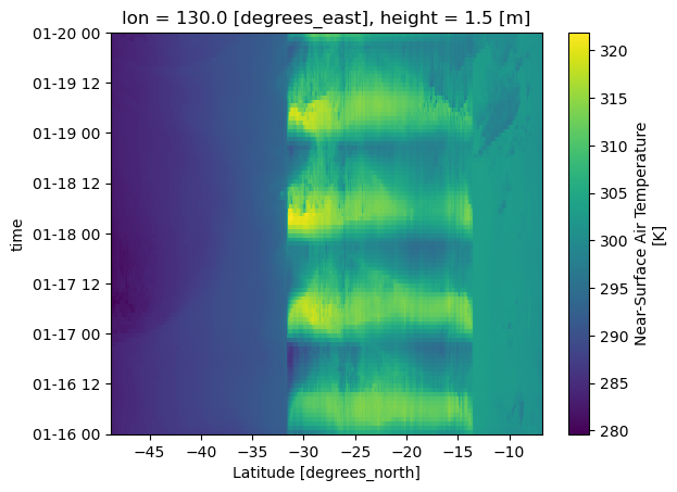
Plot a Hovmoller

tas.cf.sel(longitude = 130, method='nearest').plot()

<matplotlib.collections.QuadMesh at 0x15271aea5310>