Destaggering U and V wind components
Introduction and aims
Atmospheric models are often run on a “staggered” grid for computational stability. That is, some model variables are offset by half a grid length relative to other variables.
This includes the ACCESS model and AUS2200. In the case of AUS2200, U and V wind components have been saved on their staggered grids, and therefore need to be de-staggered prior to analysis.
This notebook demonstrates two simple methods for destaggering U and V wind components from AUS2200 data, and visualises the output with a quiver plot.
[1]:
#Assumes access to xp65 conda environment

import xarray as xr
import matplotlib.pyplot as plt
import cartopy.crs as ccrs
import numpy as np
from dask.distributed import Client
[2]:
#Start a distributed dask client. You can click "Launch dashboard in JupyterLab" in the cell output to see progress

client = Client(threads_per_worker=1)
client
[2]:
Client
Client-c7d89de2-4f66-11f1-9282-0000018dfe80
| Connection method: Cluster object | Cluster type: distributed.LocalCluster |
| Dashboard: /proxy/8787/status |
Cluster Info
LocalCluster
228737ae
| Dashboard: /proxy/8787/status | Workers: 48 |
| Total threads: 48 | Total memory: 188.56 GiB |
| Status: running | Using processes: True |
Scheduler Info
Scheduler
Scheduler-d3538f15-ced1-4be4-ac60-cedc51d359b4
| Comm: tcp://127.0.0.1:32851 | Workers: 0 |
| Dashboard: /proxy/8787/status | Total threads: 0 |
| Started: Just now | Total memory: 0 B |
Workers
Worker: 0
| Comm: tcp://127.0.0.1:37321 | Total threads: 1 |
| Dashboard: /proxy/44525/status | Memory: 3.93 GiB |
| Nanny: tcp://127.0.0.1:36287 | |
| Local directory: /jobfs/168324491.gadi-pbs/dask-scratch-space/worker-v0bdpjow | |
Worker: 1
| Comm: tcp://127.0.0.1:41871 | Total threads: 1 |
| Dashboard: /proxy/45795/status | Memory: 3.93 GiB |
| Nanny: tcp://127.0.0.1:45717 | |
| Local directory: /jobfs/168324491.gadi-pbs/dask-scratch-space/worker-v1cs56la | |
Worker: 2
| Comm: tcp://127.0.0.1:43881 | Total threads: 1 |
| Dashboard: /proxy/37157/status | Memory: 3.93 GiB |
| Nanny: tcp://127.0.0.1:43483 | |
| Local directory: /jobfs/168324491.gadi-pbs/dask-scratch-space/worker-5iw_knwa | |
Worker: 3
| Comm: tcp://127.0.0.1:45843 | Total threads: 1 |
| Dashboard: /proxy/45327/status | Memory: 3.93 GiB |
| Nanny: tcp://127.0.0.1:39847 | |
| Local directory: /jobfs/168324491.gadi-pbs/dask-scratch-space/worker-vktsg01k | |
Worker: 4
| Comm: tcp://127.0.0.1:37033 | Total threads: 1 |
| Dashboard: /proxy/36119/status | Memory: 3.93 GiB |
| Nanny: tcp://127.0.0.1:32993 | |
| Local directory: /jobfs/168324491.gadi-pbs/dask-scratch-space/worker-6kc4vdgu | |
Worker: 5
| Comm: tcp://127.0.0.1:39385 | Total threads: 1 |
| Dashboard: /proxy/39343/status | Memory: 3.93 GiB |
| Nanny: tcp://127.0.0.1:43443 | |
| Local directory: /jobfs/168324491.gadi-pbs/dask-scratch-space/worker-egwb53mi | |
Worker: 6
| Comm: tcp://127.0.0.1:32771 | Total threads: 1 |
| Dashboard: /proxy/46839/status | Memory: 3.93 GiB |
| Nanny: tcp://127.0.0.1:44215 | |
| Local directory: /jobfs/168324491.gadi-pbs/dask-scratch-space/worker-ivedyjgc | |
Worker: 7
| Comm: tcp://127.0.0.1:43193 | Total threads: 1 |
| Dashboard: /proxy/44257/status | Memory: 3.93 GiB |
| Nanny: tcp://127.0.0.1:45563 | |
| Local directory: /jobfs/168324491.gadi-pbs/dask-scratch-space/worker-1ndcmw53 | |
Worker: 8
| Comm: tcp://127.0.0.1:34213 | Total threads: 1 |
| Dashboard: /proxy/44035/status | Memory: 3.93 GiB |
| Nanny: tcp://127.0.0.1:42067 | |
| Local directory: /jobfs/168324491.gadi-pbs/dask-scratch-space/worker-io8ofjnj | |
Worker: 9
| Comm: tcp://127.0.0.1:45149 | Total threads: 1 |
| Dashboard: /proxy/42141/status | Memory: 3.93 GiB |
| Nanny: tcp://127.0.0.1:40209 | |
| Local directory: /jobfs/168324491.gadi-pbs/dask-scratch-space/worker-ah09jqx8 | |
Worker: 10
| Comm: tcp://127.0.0.1:33149 | Total threads: 1 |
| Dashboard: /proxy/45519/status | Memory: 3.93 GiB |
| Nanny: tcp://127.0.0.1:45365 | |
| Local directory: /jobfs/168324491.gadi-pbs/dask-scratch-space/worker-yop498wv | |
Worker: 11
| Comm: tcp://127.0.0.1:42891 | Total threads: 1 |
| Dashboard: /proxy/41301/status | Memory: 3.93 GiB |
| Nanny: tcp://127.0.0.1:40437 | |
| Local directory: /jobfs/168324491.gadi-pbs/dask-scratch-space/worker-as2awjr1 | |
Worker: 12
| Comm: tcp://127.0.0.1:32917 | Total threads: 1 |
| Dashboard: /proxy/36903/status | Memory: 3.93 GiB |
| Nanny: tcp://127.0.0.1:46135 | |
| Local directory: /jobfs/168324491.gadi-pbs/dask-scratch-space/worker-0po_lfu4 | |
Worker: 13
| Comm: tcp://127.0.0.1:34699 | Total threads: 1 |
| Dashboard: /proxy/41617/status | Memory: 3.93 GiB |
| Nanny: tcp://127.0.0.1:37891 | |
| Local directory: /jobfs/168324491.gadi-pbs/dask-scratch-space/worker-hsj0qks6 | |
Worker: 14
| Comm: tcp://127.0.0.1:34823 | Total threads: 1 |
| Dashboard: /proxy/39553/status | Memory: 3.93 GiB |
| Nanny: tcp://127.0.0.1:40917 | |
| Local directory: /jobfs/168324491.gadi-pbs/dask-scratch-space/worker-92xbrajq | |
Worker: 15
| Comm: tcp://127.0.0.1:44745 | Total threads: 1 |
| Dashboard: /proxy/34759/status | Memory: 3.93 GiB |
| Nanny: tcp://127.0.0.1:43045 | |
| Local directory: /jobfs/168324491.gadi-pbs/dask-scratch-space/worker-b_hxggu8 | |
Worker: 16
| Comm: tcp://127.0.0.1:36337 | Total threads: 1 |
| Dashboard: /proxy/37025/status | Memory: 3.93 GiB |
| Nanny: tcp://127.0.0.1:34327 | |
| Local directory: /jobfs/168324491.gadi-pbs/dask-scratch-space/worker-_ka8afmt | |
Worker: 17
| Comm: tcp://127.0.0.1:38381 | Total threads: 1 |
| Dashboard: /proxy/39485/status | Memory: 3.93 GiB |
| Nanny: tcp://127.0.0.1:40319 | |
| Local directory: /jobfs/168324491.gadi-pbs/dask-scratch-space/worker-dty2czrq | |
Worker: 18
| Comm: tcp://127.0.0.1:39807 | Total threads: 1 |
| Dashboard: /proxy/34679/status | Memory: 3.93 GiB |
| Nanny: tcp://127.0.0.1:45193 | |
| Local directory: /jobfs/168324491.gadi-pbs/dask-scratch-space/worker-rspqfct7 | |
Worker: 19
| Comm: tcp://127.0.0.1:43599 | Total threads: 1 |
| Dashboard: /proxy/39469/status | Memory: 3.93 GiB |
| Nanny: tcp://127.0.0.1:33073 | |
| Local directory: /jobfs/168324491.gadi-pbs/dask-scratch-space/worker-r726wh12 | |
Worker: 20
| Comm: tcp://127.0.0.1:33317 | Total threads: 1 |
| Dashboard: /proxy/44625/status | Memory: 3.93 GiB |
| Nanny: tcp://127.0.0.1:42855 | |
| Local directory: /jobfs/168324491.gadi-pbs/dask-scratch-space/worker-zpo8_nd5 | |
Worker: 21
| Comm: tcp://127.0.0.1:36873 | Total threads: 1 |
| Dashboard: /proxy/44089/status | Memory: 3.93 GiB |
| Nanny: tcp://127.0.0.1:46181 | |
| Local directory: /jobfs/168324491.gadi-pbs/dask-scratch-space/worker-nyob7twx | |
Worker: 22
| Comm: tcp://127.0.0.1:38573 | Total threads: 1 |
| Dashboard: /proxy/34059/status | Memory: 3.93 GiB |
| Nanny: tcp://127.0.0.1:33097 | |
| Local directory: /jobfs/168324491.gadi-pbs/dask-scratch-space/worker-hj3ob8h3 | |
Worker: 23
| Comm: tcp://127.0.0.1:39619 | Total threads: 1 |
| Dashboard: /proxy/37733/status | Memory: 3.93 GiB |
| Nanny: tcp://127.0.0.1:40259 | |
| Local directory: /jobfs/168324491.gadi-pbs/dask-scratch-space/worker-xp2fw8re | |
Worker: 24
| Comm: tcp://127.0.0.1:45209 | Total threads: 1 |
| Dashboard: /proxy/45395/status | Memory: 3.93 GiB |
| Nanny: tcp://127.0.0.1:36555 | |
| Local directory: /jobfs/168324491.gadi-pbs/dask-scratch-space/worker-84js7ri5 | |
Worker: 25
| Comm: tcp://127.0.0.1:46519 | Total threads: 1 |
| Dashboard: /proxy/42981/status | Memory: 3.93 GiB |
| Nanny: tcp://127.0.0.1:46197 | |
| Local directory: /jobfs/168324491.gadi-pbs/dask-scratch-space/worker-y67z72wk | |
Worker: 26
| Comm: tcp://127.0.0.1:38971 | Total threads: 1 |
| Dashboard: /proxy/36031/status | Memory: 3.93 GiB |
| Nanny: tcp://127.0.0.1:33545 | |
| Local directory: /jobfs/168324491.gadi-pbs/dask-scratch-space/worker-zh_v4pce | |
Worker: 27
| Comm: tcp://127.0.0.1:33249 | Total threads: 1 |
| Dashboard: /proxy/44521/status | Memory: 3.93 GiB |
| Nanny: tcp://127.0.0.1:46191 | |
| Local directory: /jobfs/168324491.gadi-pbs/dask-scratch-space/worker-yu613f5d | |
Worker: 28
| Comm: tcp://127.0.0.1:35155 | Total threads: 1 |
| Dashboard: /proxy/39723/status | Memory: 3.93 GiB |
| Nanny: tcp://127.0.0.1:44441 | |
| Local directory: /jobfs/168324491.gadi-pbs/dask-scratch-space/worker-59133i0l | |
Worker: 29
| Comm: tcp://127.0.0.1:40905 | Total threads: 1 |
| Dashboard: /proxy/39683/status | Memory: 3.93 GiB |
| Nanny: tcp://127.0.0.1:39163 | |
| Local directory: /jobfs/168324491.gadi-pbs/dask-scratch-space/worker-vwbnlvou | |
Worker: 30
| Comm: tcp://127.0.0.1:34449 | Total threads: 1 |
| Dashboard: /proxy/44535/status | Memory: 3.93 GiB |
| Nanny: tcp://127.0.0.1:41663 | |
| Local directory: /jobfs/168324491.gadi-pbs/dask-scratch-space/worker-c9xnavlm | |
Worker: 31
| Comm: tcp://127.0.0.1:35609 | Total threads: 1 |
| Dashboard: /proxy/42051/status | Memory: 3.93 GiB |
| Nanny: tcp://127.0.0.1:38267 | |
| Local directory: /jobfs/168324491.gadi-pbs/dask-scratch-space/worker-wqypn0j4 | |
Worker: 32
| Comm: tcp://127.0.0.1:36557 | Total threads: 1 |
| Dashboard: /proxy/34965/status | Memory: 3.93 GiB |
| Nanny: tcp://127.0.0.1:35097 | |
| Local directory: /jobfs/168324491.gadi-pbs/dask-scratch-space/worker-xf4nymf0 | |
Worker: 33
| Comm: tcp://127.0.0.1:42291 | Total threads: 1 |
| Dashboard: /proxy/33997/status | Memory: 3.93 GiB |
| Nanny: tcp://127.0.0.1:35331 | |
| Local directory: /jobfs/168324491.gadi-pbs/dask-scratch-space/worker-u9cdyfgb | |
Worker: 34
| Comm: tcp://127.0.0.1:39065 | Total threads: 1 |
| Dashboard: /proxy/42245/status | Memory: 3.93 GiB |
| Nanny: tcp://127.0.0.1:40321 | |
| Local directory: /jobfs/168324491.gadi-pbs/dask-scratch-space/worker-3ytel2xm | |
Worker: 35
| Comm: tcp://127.0.0.1:42157 | Total threads: 1 |
| Dashboard: /proxy/46721/status | Memory: 3.93 GiB |
| Nanny: tcp://127.0.0.1:34611 | |
| Local directory: /jobfs/168324491.gadi-pbs/dask-scratch-space/worker-9ssrekzz | |
Worker: 36
| Comm: tcp://127.0.0.1:34945 | Total threads: 1 |
| Dashboard: /proxy/36171/status | Memory: 3.93 GiB |
| Nanny: tcp://127.0.0.1:34203 | |
| Local directory: /jobfs/168324491.gadi-pbs/dask-scratch-space/worker-yv823uv2 | |
Worker: 37
| Comm: tcp://127.0.0.1:43649 | Total threads: 1 |
| Dashboard: /proxy/46569/status | Memory: 3.93 GiB |
| Nanny: tcp://127.0.0.1:38269 | |
| Local directory: /jobfs/168324491.gadi-pbs/dask-scratch-space/worker-_s9o8et2 | |
Worker: 38
| Comm: tcp://127.0.0.1:36187 | Total threads: 1 |
| Dashboard: /proxy/38273/status | Memory: 3.93 GiB |
| Nanny: tcp://127.0.0.1:44281 | |
| Local directory: /jobfs/168324491.gadi-pbs/dask-scratch-space/worker-z5e5_ywv | |
Worker: 39
| Comm: tcp://127.0.0.1:37441 | Total threads: 1 |
| Dashboard: /proxy/44563/status | Memory: 3.93 GiB |
| Nanny: tcp://127.0.0.1:45421 | |
| Local directory: /jobfs/168324491.gadi-pbs/dask-scratch-space/worker-e37h5bm7 | |
Worker: 40
| Comm: tcp://127.0.0.1:37591 | Total threads: 1 |
| Dashboard: /proxy/45891/status | Memory: 3.93 GiB |
| Nanny: tcp://127.0.0.1:44923 | |
| Local directory: /jobfs/168324491.gadi-pbs/dask-scratch-space/worker-qbe8c0_8 | |
Worker: 41
| Comm: tcp://127.0.0.1:34329 | Total threads: 1 |
| Dashboard: /proxy/43831/status | Memory: 3.93 GiB |
| Nanny: tcp://127.0.0.1:46689 | |
| Local directory: /jobfs/168324491.gadi-pbs/dask-scratch-space/worker-8feufdos | |
Worker: 42
| Comm: tcp://127.0.0.1:41001 | Total threads: 1 |
| Dashboard: /proxy/38603/status | Memory: 3.93 GiB |
| Nanny: tcp://127.0.0.1:36993 | |
| Local directory: /jobfs/168324491.gadi-pbs/dask-scratch-space/worker-ik_qqnzs | |
Worker: 43
| Comm: tcp://127.0.0.1:46307 | Total threads: 1 |
| Dashboard: /proxy/41845/status | Memory: 3.93 GiB |
| Nanny: tcp://127.0.0.1:43893 | |
| Local directory: /jobfs/168324491.gadi-pbs/dask-scratch-space/worker-mpwqkwsh | |
Worker: 44
| Comm: tcp://127.0.0.1:32815 | Total threads: 1 |
| Dashboard: /proxy/45881/status | Memory: 3.93 GiB |
| Nanny: tcp://127.0.0.1:33583 | |
| Local directory: /jobfs/168324491.gadi-pbs/dask-scratch-space/worker-v7xo_cgv | |
Worker: 45
| Comm: tcp://127.0.0.1:42649 | Total threads: 1 |
| Dashboard: /proxy/38001/status | Memory: 3.93 GiB |
| Nanny: tcp://127.0.0.1:40091 | |
| Local directory: /jobfs/168324491.gadi-pbs/dask-scratch-space/worker-8pfbplf0 | |
Worker: 46
| Comm: tcp://127.0.0.1:40465 | Total threads: 1 |
| Dashboard: /proxy/39035/status | Memory: 3.93 GiB |
| Nanny: tcp://127.0.0.1:34171 | |
| Local directory: /jobfs/168324491.gadi-pbs/dask-scratch-space/worker-prqxdwyj | |
Worker: 47
| Comm: tcp://127.0.0.1:36411 | Total threads: 1 |
| Dashboard: /proxy/46561/status | Memory: 3.93 GiB |
| Nanny: tcp://127.0.0.1:42789 | |
| Local directory: /jobfs/168324491.gadi-pbs/dask-scratch-space/worker-vsr92sww | |
[4]:
# Lets use intake to grab a couple of AUS2200 files to play with
import intake


datastore = intake.cat.access_nri["AUS2200"]
datastore = datastore.search(realm='atmos')
datastore = datastore.search(experiment_id='ecoastlow-evolvsst')
datastore = datastore.search(frequency='1hr')
datastore = datastore.search(variable_id=["uas","vas"])

uas = datastore.search(variable_id="uas").to_dask(xarray_open_kwargs={'chunks' : {}})
vas = datastore.search(variable_id="vas").to_dask(xarray_open_kwargs={'chunks' : {}})
[5]:
uas = uas.sel(time='2016-06-05 18:00',method="nearest").squeeze()
vas = vas.sel(time='2016-06-05 18:00',method="nearest").squeeze()
[6]:
print("Experiment description: \n")
print(uas.attrs["exp_description"])
Experiment description:

A limited area model study of the entire Australian continent at 2.2 km resolution, using the UM atmospheric model. ERA5+ERA5Land reanalysis data was used to provide initial and boundary conditions, sea-surface temperatures are evolving throughout the simulation. The study covers the period from 2016-06-03 to 2016-06-07, including the East Coast Low event which gave rise to widespread flooding in many areas stretching from southeast Queensland, eastern New South Wales, eastern Victoria, and large areas of northern Tasmania.
You can see more information on this runs, including how to cite it,here
Chunking
We have loaded in in 10-metre u and v wind data, with 4 chunks in the lat and lon directions. We will return to this later when we consider different destaggering methods
[7]:
uas.uas
[7]:
<xarray.DataArray 'uas' (lat: 2120, lon: 2600)> Size: 22MB
dask.array<getitem, shape=(2120, 2600), dtype=float32, chunksize=(1060, 1300), chunktype=numpy.ndarray>
Coordinates:
  * lat      (lat) float64 17kB -48.79 -48.77 -48.75 ... -6.871 -6.852 -6.832
  * lon      (lon) float64 21kB 114.3 114.3 114.3 114.3 ... 165.7 165.7 165.7
    time     datetime64[ns] 8B 2016-06-05T18:30:00.000000256
    height   float64 8B ...
Attributes:
    standard_name:          eastward_wind
    long_name:              Eastward Near-Surface Wind
    comment:                Eastward component of the near-surface (usually, ...
    units:                  m s-1
    cell_methods:           area: mean time: mean
    cell_measures:          area: areacella
    history:                2024-10-16T01:32:52Z altered by CMOR: Treated sca...
coverage_content_type: modelResultStaggered grid
The AUS2200 u wind data has been saved on a staggered longitude grid, while the v wind data has been saved on a staggered latitude grid. See how the longitude coordinates are different (and offset by 0.5 * grid spacing). If we were to combine u and v now into one dataset using something like xr.Dataset({"u":uas.uas,"v":vas:vas}), then xarray would do it by meshing together the grids with missing values (this is not what we want to do).
[8]:
vas.lon.isel(lon=slice(0,20)).plot(marker="o")
uas.lon.isel(lon=slice(0,20)).plot(marker="o")
plt.gca().grid(ls=":")
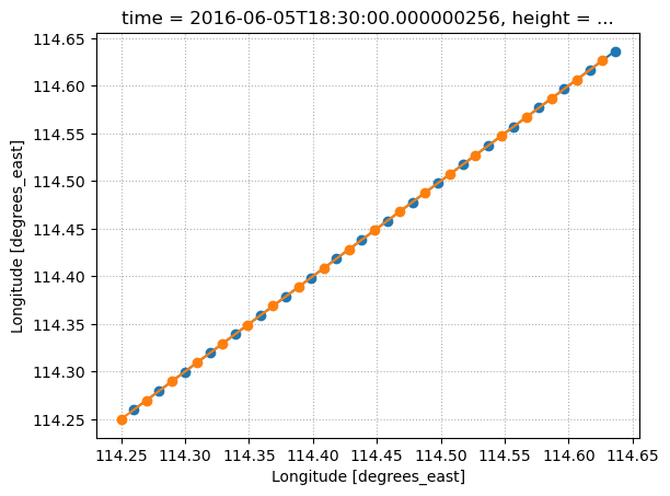
The staggered grid has also resulted in one extra latitude grid point, so the vas variable is on a different size grid
[9]:
uas.uas.shape
[9]:
(2120, 2600)
[10]:
vas.vas.shape
[10]:
(2121, 2600)
Destaggering (centring)
If we want to perform any analysis or make plots, we need u and v to be on the same grid. Our first method will be to centre u in longitude and v in latitude by averaging
[11]:
#Set up the destaggered coordinates.
#Note that our centring approach will result in one less grid point, so we need to slice the lons down accordingly
#The latitude for v is already one grid point longer than u, so we don't need to do this for latitude

destaggered_lon_coord = vas.lon.isel({"lon":slice(0,-1)})
destaggered_lat_coord = uas.lat
[12]:
#Now we can slice and centre/average the U data in longitude.
#We need to manually reassign the longitude coordinates using assign_coords()
uas_destaggered = ((uas.uas.isel({"lon":slice(0,-1)}).assign_coords({"lon":destaggered_lon_coord}) +\
      uas.uas.isel({"lon":slice(1,uas.lon.shape[0])}).assign_coords({"lon":destaggered_lon_coord})) / 2)
[13]:
#Same for V
vas_destaggered = ((vas.vas.isel({"lat":slice(0,-1)}).assign_coords({"lat":destaggered_lat_coord}) +\
      vas.vas.isel({"lat":slice(1,vas.lat.shape[0])}).assign_coords({"lat":destaggered_lat_coord})) / 2)
Combining
Now we can safely combine the u and v wind components into one dataset (useful for plotting later), and calculate wind speed.
Note that out chunking has been preserved in this method
[14]:
destaggered_ds = xr.Dataset({"u":uas_destaggered,"v":vas_destaggered})
destaggered_ds["wind_speed"] = np.sqrt( destaggered_ds["u"]**2 + destaggered_ds["v"]**2 )
[15]:
destaggered_ds["u"]
[15]:
<xarray.DataArray 'u' (lat: 2120, lon: 2600)> Size: 22MB
dask.array<where, shape=(2120, 2600), dtype=float32, chunksize=(1060, 866), chunktype=numpy.ndarray>
Coordinates:
  * lat      (lat) float64 17kB -48.79 -48.77 -48.75 ... -6.871 -6.852 -6.832
  * lon      (lon) float64 21kB 114.3 114.3 114.3 114.3 ... 165.7 165.7 165.7
    time     datetime64[ns] 8B 2016-06-05T18:30:00.000000256
    height   float64 8B 10.0
Attributes:
    standard_name:          eastward_wind
    long_name:              Eastward Near-Surface Wind
    comment:                Eastward component of the near-surface (usually, ...
    units:                  m s-1
    cell_methods:           area: mean time: mean
    cell_measures:          area: areacella
    history:                2024-10-16T01:32:52Z altered by CMOR: Treated sca...
coverage_content_type: modelResultDestaggering (interp)
It would be a little neater to just use xr.interp to destagger, which is demonstrated below. But note that our chunking is not preserved in this method, because dask needs to access the whole lat/lon dimension to do the spatial interpolation. So we now have only one chunk in longitude for the U variable. This is an important consideration if you need to destagger on really large data (not an issue here for one time step, and surface level data only)
[16]:
uas_destaggered_interp = uas.uas.interp({"lon":destaggered_lon_coord},method="linear")
vas_destaggered_interp = vas.vas.interp({"lat":destaggered_lat_coord},method="linear")
destaggered_ds_interp = xr.Dataset({"u":uas_destaggered_interp,"v":vas_destaggered_interp})
destaggered_ds_interp["wind_speed"] = np.sqrt( destaggered_ds_interp["u"]**2 + destaggered_ds_interp["v"]**2 )
destaggered_ds_interp["u"]
[16]:
<xarray.DataArray 'u' (lat: 2120, lon: 2600)> Size: 22MB
dask.array<where, shape=(2120, 2600), dtype=float32, chunksize=(530, 2599), chunktype=numpy.ndarray>
Coordinates:
  * lat      (lat) float64 17kB -48.79 -48.77 -48.75 ... -6.871 -6.852 -6.832
  * lon      (lon) float64 21kB 114.3 114.3 114.3 114.3 ... 165.7 165.7 165.7
    time     datetime64[ns] 8B 2016-06-05T18:30:00.000000256
    height   float64 8B 10.0
Attributes:
    standard_name:          eastward_wind
    long_name:              Eastward Near-Surface Wind
    comment:                Eastward component of the near-surface (usually, ...
    units:                  m s-1
    cell_methods:           area: mean time: mean
    cell_measures:          area: areacella
    history:                2024-10-16T01:32:52Z altered by CMOR: Treated sca...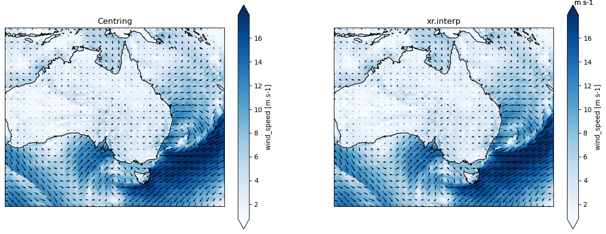
coverage_content_type: modelResultPlotting
Visualise the winds using a quiver plot and contour the wind speed. Both methods of destaggering produce the same outcome
[17]:
#Set the spacing of the wind vectors in lat and lon
step = 75

plt.figure(figsize=[16,6])
ax = plt.subplot(1,2,1,projection=ccrs.PlateCarree())
destaggered_ds["wind_speed"].plot(robust=True,cmap="Blues")
destaggered_ds.isel({"lat":slice(0,-1,step),"lon":slice(0,-1,step)}).plot.quiver(
    "lon","lat","u","v")
ax.coastlines()
plt.title("Centring")

ax = plt.subplot(1,2,2,projection=ccrs.PlateCarree())
destaggered_ds_interp["wind_speed"].plot(robust=True,cmap="Blues")
destaggered_ds_interp.isel({"lat":slice(0,-1,step),"lon":slice(0,-1,step)}).plot.quiver(
    "lon","lat","u","v")
ax.coastlines()
plt.title("xr.interp")
[17]:
Text(0.5, 1.0, 'xr.interp')
Contributors
Andrew Brown
ARC Centre of Excellence for 21st Century Weather, University of Melbourne
Charles Turner
ACCESS-NRI, Australian National University, Canberra
If you have any enquries, suggested improvements or bug reports related to this recipe, please open an issue or start a discussion in this repository.